ProcMT and SW

ProcMT main GUI

Basic application video:

(click video to full screen)

Tab dirs

drag & drop the toplevel directory on “survey base dir” or use the select button

For emap, local & center and remote reference prefer the select button, which open sites belonging to this “survey base dir”.

Tab settings

cut upper f, cut lower f

Determines the usable part of the FFT.
If too small less frequencies for each band will be used; overlapping bewteen bands is reduced

ProcMT preference

smooth takes in general shorter FFTs and bigger parzening

medium takes most common settings

sharp takes longer FFTs and smaller parzening

auto bandwidth, auto Parzen

You can tune the “ProcMT preference” by changing these values.
I happens that - for example “sharp” is selected, a bigger parzen radius gives the desired result

skip marked parts

If a selection in the timerseries has been made, respect this and exclude these parts from beeing read.

Tab MT

THE WORKFLOW is

• calculate Z tensor
• perform a quadrant check
• check the coherency
• range check by median of rho and phi for xy, yx
• statistical evaluation of the selected data
• if “stddev limit active”, take all values with standard deviation less than “x std dev”
• if stddev limit active AND stddev auto is active, take all values with standard deviation less than and iterative lower the limit to “x std dev min”; breaks if less than 32 stacks automatically
• again a final statistical evaluation of the selected data follows

quadrant check

In most cases you expect the relation that real and imaginary part of Zxy (Ex, Hy) are positive and Zyx (Ey, Hx) are negative. There may be complex 3D cases where this is not the case. So this option is not “fail safe”.
However in the spectral editor you can look at this distribution. Normally if Zxy is mostly positive the negative elements represent outliers which appear as “wrong phase”. If checked negative Zxy will be treated as outliers. This tensor will be removed from the statistics.

ProcMT RR with an AMT Site

Especially when using the MFS-06e coils you can enhance the data above 1 kHz by doing remote referencing (RR) with a station nearby.
Here the dominating effect is the self noise reduction by using H :sub:x*H :sub:xr instead of H :sub:x*H :sub:x and so on (so cross spectra instead of auto spectra)

RR with AMT Site:

(click video to full screen)

ProcMT Join AMT RR Site and MT Site

This procedure applies for any type of processing; you can merge / edit / delete any combination. In the later case we mix the LF part of and EDI with the HF part (processed with RR)

RR AMT and MT Site:

(click video to full screen)

ProcMT Export to SQLite, Matlab, Octave, R and Python

All the above programming languages can read SQL databases, including the SQLite database.
ProcMT can write and read SQLite files. File size is around 20 x smaller compared to single ASCII files and all is together in one file.

So if you focus on mathematics only, your Matlab experiments may be included in our processing if you find it valuable.

ProcMT spectra export and import:

(click video to full screen)

Cal2SQL

get calibration

Fetch a coil from the database for plotting

OpenCreate

You may want to create your output directory first, like allcoils and click that directory. |br| Give a name like coils.sql3 |br| You will be prompted for an output directory - cal2sql will later immediately write without prompting. |br| Drag & drop yout txt file onto the window and the database will be filled.

Stats

FIRST select coil type and press “get calibration”. |br| AFTER this you can press Stats. Additionally a CSV table with the statistical results will be written on the fly.

FAQ ProcMT

I do not get all frequencies

At the lower end: you FTT / window length is too short.
The time series is too short, and ProcMT does not find a reasonable solution. Hence that this also applies to stack all.
In settings you can a) tick “sharp” in order to get a longer FFT or b) manually by ticking “off” and select the window length manually. If you don’t want to re-process all data, go to the “Freqs” tab and select/deselect the frequencies to be processed.
The above changes may give more frequencies in th EDI result - if the data is good or medium quality.
In case the recording was long enough it may also work with “smooth” and/or “off” & shorter FFT. In this case ProcMT has rejected too many stacks with the longer FFT and can not make a statistics. Using a shorter FFT leads to more stacks and possibly to a reasonable statistics.

If the data quality is not so good, you may want to find out, what a “stack all” may give you.
In the “MT” Tab you can uncheck quadrant check.
Additionally you can lower the “coherency threshold” to 0.4 or uncheck “ct active”. Press “reset tensor” and “re-calculate tensor”.
The result may look awkward - but contains more / all frequencies.

For all these problems read again the chapter below.

See also Why do I need to stack timeseries

On the upper end: FFT too short.
Calibration stops at 10 kHZ and you want to see 30 kHz
Can’t see 10 kHz: parzening needs some upper frequencies, so e.g. you get 8 kHz for the MFS-06e.
Short FFT and small parzening causes the same problem.

Change the Target Frequencies

The default setting is 8 frequencies per decade. Since MT has a smooth transfer function a higher resolution does not add information.
However it may be necessary to change the list in order to fit with other projects.

Inside the ProcMT directory you find “info.sql3” - that is a SQLite database. On Mac/Linux/Windows you can (after making a copy) edit this file with SQLiteBrowser

You find 6 tables user[123]_mt_frequencies and user[123]_csem_frequencies which are reserved for editing. You can put a descending frequency list inside.
The procmt_mini will be able to load them. Hint : procmt_mini can be called with two parameters: -basedir /survey/mining and/or -target_frequencies_table user1_mt_frequencies … and so on
That way you fasten the GUI operation; create a desktop icon for example, containing these parameters.

@superuser create a file called user1_mt_frequencies.csv; put “frequencies” in line 1, then your frequencies; delete user1_mt_frequencies in info.sql3; import your csv

The csv file will be a single column file like below.

frequencies
8.00000000000000E+05
5.99600000000000E+05
…

@programmer’s note: procmt has to handle data on four different OS; SQLite is a stable solution. Text files not.

Survey Folder Structure

ProcMT and other programs rely on a certain directory structure.

survey name	subdirectory	site
Northern mining
	cal
	config
	db
	dump
	edi
	filters
	jle
	jobs
	log
	processings
	shell
	tmp
	ts
	… inside ts:
		EW 12 L2
		EW 14 L2
		EW 17 L2
		Remote Green Valley
		大仏山

… and so on

structure

If you don’t have and do not work with ProcMT, you may want to create it temporarily in order to work with all modules which rely on the structure.
A litte PHP script can do that:

#!/usr/bin/php
<?php
$subdirs = array("cal", "config", "db", "dump", "edi", "filters", "jle", "jobs", "log", "processings", "shell", "tmp", "ts");
#
#
if ($argc < 2 ) {
    exit( "Usage: $argv[0] folder_name" . PHP_EOL );
}
else {
 if (!is_dir("$argv[1]") ) mkdir("$argv[1]");
}
#
if (is_dir("$argv[1]")) {
  foreach ($subdirs as $subdir) {
    $cdir = "$argv[1]" . "/" . "$subdir";
    echo "creating " . $cdir . PHP_EOL;
    if (!is_dir("$cdir") ) mkdir("$cdir");
  }
}
#
?>

cal

Inside the cal directory you copy your calibration files in case.
If you have a ADU-07e, ADU-08e AND MFS-0Xe coils (or sensors ending with “e”) you do not need to do that. In the measdoc.xml you will find the calibration data of the connected sensors:

<channel id="2">
 <calibration>
   <cal_version>1.0</cal_version>
   <creator>software chcal 1.3</creator>
   <user>metronix</user>
   <calibrated_item>
     <ci identifier="coil">MFS06e</ci>
     <ci_serial_number>4774</ci_serial_number>
      .....


   <caldata chopper="on" gain_2="0" gain_3="0" gain_1="0" impedance="(0,0)">
     <c0 unit="V">0.00000000e+00</c0>
     <c1 unit="Hz">1.87380000e-01</c1>
     <c2 unit="V/(nT*Hz)">1.99940000e-01</c2>
     <c3 unit="deg">8.72760000e+01</c3>
   </caldata>

   ...

which indicates the calibration was loaded.
OTHERWISE you copy the delivered calibration file into the cal directory.

A typical calibration file has the name MFS06026.TXT and contains:

Calibration measurement with Solartron
Metronix GmbH, Kocherstr. 3, 38120 Braunschweig

Magnetometer: 026    Date: 06/12/01    Time: 11:23:02


FREQUENCY    MAGNITUDE      PHASE    
    Hz                     deg 
Chopper On       
+1.0000E-01  +2.0027E-01  +8.8566E+01   
+1.2589E-01  +1.9994E-01  +8.8187E+01   
+1.5849E-01  +2.0034E-01  +8.7711E+01   
+1.9953E-01  +1.9996E-01  +8.7177E+01   

.....

+7.9430E+03  +6.9484E-05  -4.0999E+01   
+9.9995E+03  +5.1712E-05  -5.1017E+01   
+1.0000E+04  +5.1707E-05  -5.1019E+01   

FREQUENCY    MAGNITUDE      PHASE      
    Hz                     deg          
Chopper Off    
+1.0000E+00  +1.8154E-01  +1.1703E+02   
+1.2589E+00  +1.9576E-01  +1.0632E+02   
+1.5849E+00  +2.0317E-01  +9.5114E+01   
+1.9953E+00  +2.0268E-01  +8.3716E+01   
+2.5119E+00  +1.9471E-01  +7.2457E+01   

....

config

In case onfiguration files for special processings

db

Databases - e.g. coil calibration databases, EDI databases

dump

dump files (spectra, applied calibration) in case dump mode activated

filters

empty

jle

Job List Editor - for putting your xml joblists for this survey here

jobs

actual xml jobs running or xml jobs to be run in the future
for example: create 100 jobs and run them over night

log

log files in case created

processings

pre-defined processings to submit

shell

shell scripts or PHP scripts

tmp

temporary files

ts

contains your sites and your timeseries
HINT even if you have downloaded a single folder like “meas_2018-10-20_09-50-00”, you MUST create a site first say test and copy meas_2018-10-20_09-50-00 into test.

atsfilter

The default filter is 4x decimation. And the default spacing of frequencies is 16x. By filtering each recording with 4x you get a continuous set of bands with 4x spacing - that is the idea (How long do I have to record?
The drag & drop scans xml files recursive: you can drag & and drop several measdirs or even the complete site. Sure: for cutting you drop only one xml file (mostly).

The major purpose is to down filter the timeseries. By filtering you get lower sampling frequencies (lower bands). Theoretically you achieve the similar result by increasing the FFT … but not the same result. A FIR filter (finite impulse response) in time domain ist not the same like a “longer FFT”.

filter tab

the default filter 4x is already checked.
If you have recorded for a longer time, go to the center to the Cascades scroll box and select, how many times the timerseries shall be filtered again.

Options: - auto extend: filters down to a reasonable size - Low Pass … - High Pass … - Band pass …

The notch filters can be combined in case, for example 16 2/3 & 50 & 150 Hz. DO NOT USE THEM in case you want to process the data for MT later; the only possible usage is for display data in your publication.
The filtering is done in the time domain. But it is similar to a large window FFT with removing the desired frequencies. You may sometimes see differcences in processing the data with/without filtering; but this may be related to the settings of your processing. If you take large FFT windows and small Parzen windows the results between filtered and non filtered processing converge.
Another typical mistake is to evaluate frequencies too close to the sample rate. If you take a sampling rate of 256 Hz the evaluation of 64 Hz data is sportive. ProcMT takes 64 Hz already as corner frequency.

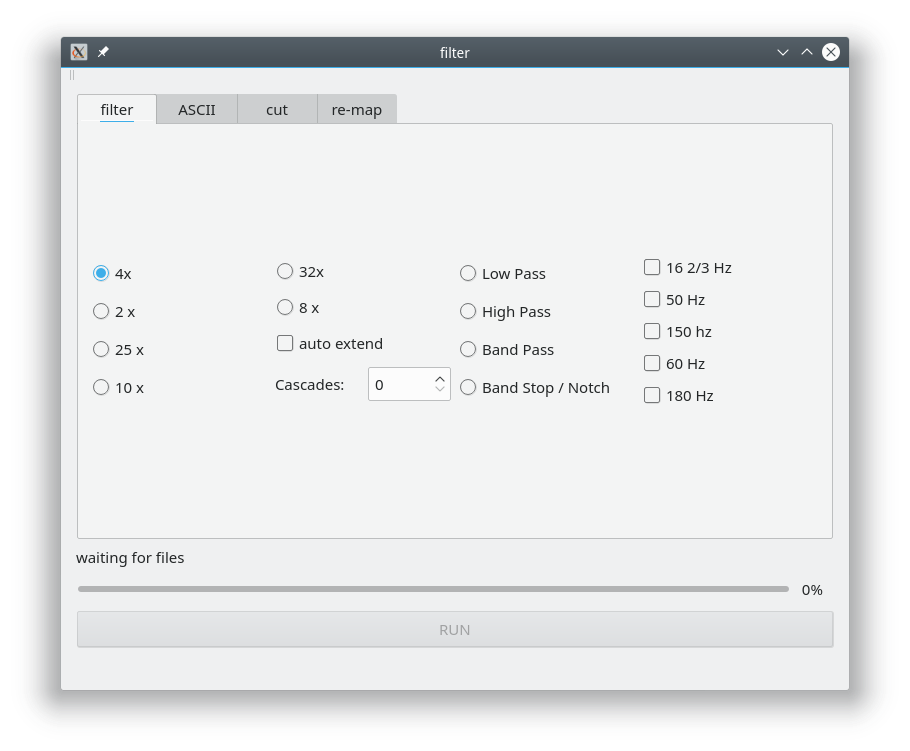
The 16 2/3 Hz 50 Hz / 150 Hz as well as the 60 Hz / 180 Hz filters can be combined.
The INPUT will not be deleted. In case of multiple filtering, temporary directories will appear shortly.
You identify the new directories by their date: the filter always has to shift by 1 s (or more for lower sampling rates); so using 50 & 150 Hz notch gives a 2 seconds shifted start time. You may want to delete the source directories manually! (You have a copy of the originals see also notes ).

Default Filtering

ASCII

(click video to full screen)

You can export to ASCII with following options:

Options:

• ASCII output -> saves data as mV
• ASCII output scaled -> scales E to mV/km -> that is the option you want
• ASCII output scaled and nT -> tries! to convert data to mV (E) and nT (H)
• ASCII output scaled and nT -> tries! to convert data to mV (E) and nT (H) using theoretical transfer function only

When using the theoretical function only - atsfilter will nevertheless load the calibration for f_sample > 512 Hz in order to avoid calibration errors.

WARNING 1

For the data in nT a full FFT inversion of ALL data is made. The FFT uses “zero padding” in order to have 2 :sup:2 values (513 values will become 1024 values).
Having 50 MB ats data we get 100MB of doubles in RAM, padded to 200 MB.
The frequency, amplitude and phase values will also have 200 MB of size; that makes 800MB. Plus temporary storage we get 1.2 GB out of 50 MB of data!

The computation time takes very long; when you have not enough memory you computer will -> swap -> freeze -> dead
On some computers the GUI may freeze - but the software still runs (check with your system load). That may be caused by 100% workload.

WARNING 2

A FFT over 100,000 data points is NOT the same like N FTTs with 1024 point over 100,000 data points.
The detrend is NOT the same. So when sections are compared you get NOT the same result and the timeseries are looking different.
Also the spectra are not the same! For the professional timeseries analysis you may use a detrend and a Hanning window in order to avoid a mapping of the window length (1024) into the spectral domain as sinc function.

Some virtual machines (VM) may break down early; also writing to the local drive via “network” may cause trouble.

The GUI seems to be not responding when the FFTs are calculated - please be patient

Conclusion

In case you know what you are doing, conversion is fine (display timeseries data).
If you compare with fluxgate data: cut the timeseries data into that segment you really want to compare.
If you want to use the inverted data for spectral processing or even magnetotelluric data … you may run into trouble.

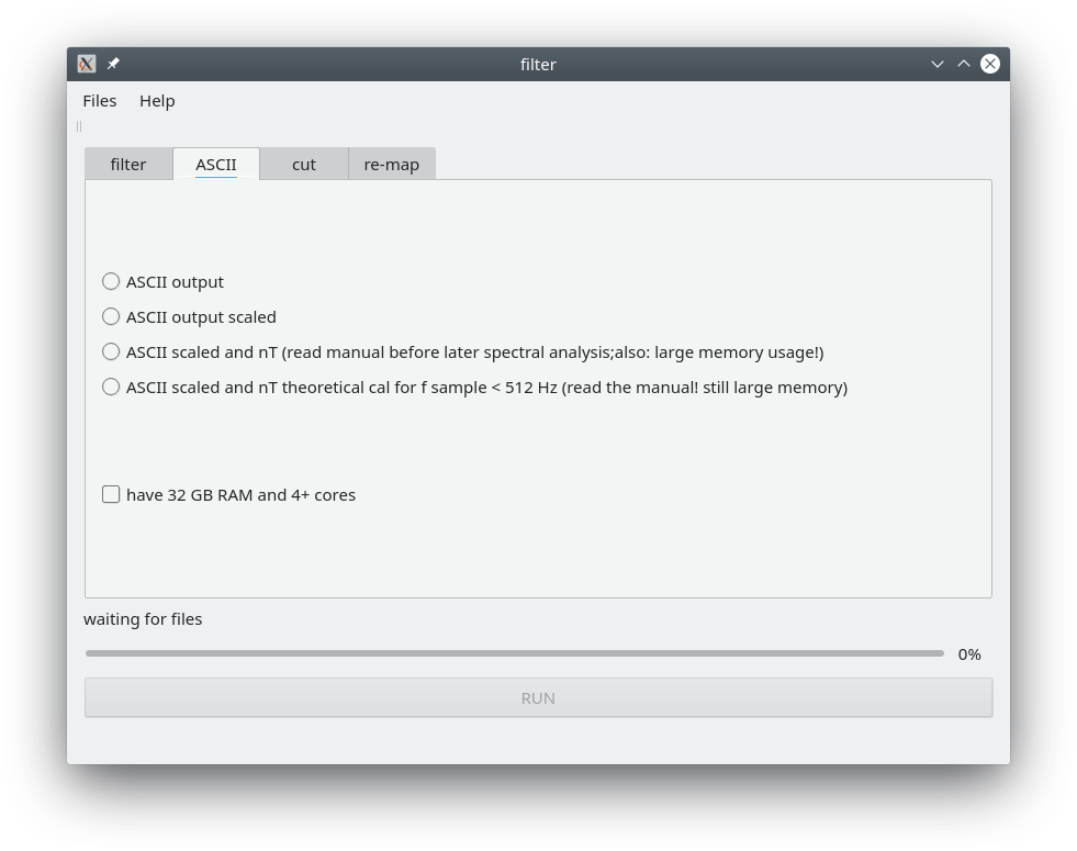
Example: dropping folders:

Band Stop Filter

Important: Band stop filtering (notch filter) does not really improve the MT result.
During the MT processing you go to the spectral domain and simply avoid to 50 Hz or 150 Hz as target frequencies.

(click video to full screen)

Cutting

Cutting allows you to modify the the recording duration. This can be useful if you know that on the last day for example the E field was chopped of and this data is for ever useless.

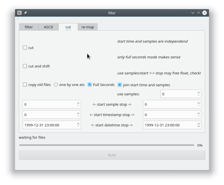
Options:

• cut : cuts from given start (time or sample) to given stop (time or sample)
• cut and shift : … not implemented yet
• copy old files If “copy old files” is checked (“cut should be activated automatically”) you can drag & drop old files from ADU-06 and ADU-07. Take always a set of 5 files.
  The procedure is quite straight forward - it will not repair any awkward settings; chopper will be set automatically.
• one by one ats : indicates that time series will not down filtered while cutting (default)
• Full seconds : if NOT checked you may be able to cut 6 samples from a 1024 Hz time series - otherwise counter will jump by 1024 (default)
• join start time and samples : try to cut and stay GPS synced

re-map

First acknowledge that your data may be inconsistent - for whatever reason; and you have made already a backup.
What is does:
Drag & Drop the XML file on top. In the ats header (ref: Programmers Notes, atsheader ) uiChanNo and achChanType will be changed. Additionally the filename will be changed. Example Hy -> Hx
3 -> 2; Hy -> Hx; 203_V01_C03_R000_THy_BL_8H.ats -> 203_V01_C03_R000_THy_BL_8H.ats
Additionally the XML file has to be re-written (re-write the part and swapping the ). That are at least the section and the section. Other parts remain untouched
Attention in case of a 5 channel file, you can not re-map a single channel logically! Also you can not create a new channel. So it is simply spoken only possible to “swap” existing channels.

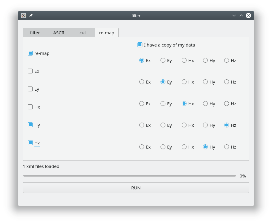
As you can see, Hy and Hz are checked and the button-matrix shows the desired action. You can drop a complete site in case ALL are 5 channels (or 4 and so on).
A sign reversal is NOT applied (dos not make West to East).

following options are available from a command line or (e.g. PHP) script in case XML files are selected (not ats files):

• -filter 4x [or 2x, 4x, 8x, 10x, 25x, 32x]
• -notch 50 [or 16_23, 50, 150, 50_150, 16_23_50_150, 60, 180, 60_180] where as 16_23 is 16 2/3 (railway frequency)
• -ascii scaled [or raw, scaled, nt, nt_theo]
• -gui false [true]
• files (measdoc files)

Since the measdoc (like 216_2018-04-20_11-57-13_2018-04-23_07-58-02_R000_16H.xml) indicates all what is need you can use (for example) a recursive PHP script in order to find which files you want to work on.
You can load many measdocs ath the same time.

If -gui true the gui will be called and you continue to work there.

Exmaple: atsfilter -ascii scaled -gui false meas_2018-04-20_11-57-13/216_2018-04-20_11-57-13_2018-04-23_07-58-02_R000_16H.xml meas_2018-04-20_12-00-00/216_2018-04-20_12-00-00_2018-04-24_07-58-02_R000_8H.xml

Script interface

notes

In the “old days” band-pass and notch filtering was used BEACAUSE the number of bits (e.g.14 or 16) where to small to digitize the MT signal including spikes (outliers).
You always (including today) you use a low pass filter which cuts of at (or before) the Nyquist frequency. If you sample with 4 kHz the low pass filter must suppress all above 4 kHz (or better 3 kHz).
In theory you can calculate a FFT up to 2 kHz now (sampling theorem). For better resolution however you go up to 1 kHz or 512 Hz. In this case you are away from the filter influence (modern delta-sigma ADC (analogue digital converter) sample at a MHz, so the low pass filter is actually higher). For the expert: with coils and fluxgate this is easy. But for the electric field we a coupled to the ground (contact resistivity) - which is a non constant system. Therefore the ADU switches additional “radio filters” to compensate that.

In the old days additional analogue high pass and low pass filters where switched (signal conditioning) in order to keep the signal range small (max/min). Behind these filters gains (analogue amplifier) were switched to feed the ADC into the optimum range. Especially you want to avoid over powering the ADC because the ADC has a relaxation time: that is the time he goes back to normal operation.
What is normally not mentioned: all these filters have a) transfer function and b) a relaxation time. a) can be neglected in case your interpretation frequencies are far away from the filter’s corner frequencies. b) however is a tragedy. If a spike (impulse) hits the filter, the filter smoothes the spike down to a long slope (where the data is ruined).
That is why the ADU systems to not use one of these filters.

The solution came with the new 24 bit and 32 bit ADCs. The max/min range is so high that the analogue filter conditioning is not needed anymore.
Removing the 50 / 60 Hz is cosmetics today. Only if the processing is not well conditioned (FFT, Parzen radius) you get influence from the powerline frequencies.

atsedit

Allows your edit the binary header of ATS files.
As long as you do not change relevant data - it is ok.
In case of changing time, date, channel number, channel type your data may become inconsistent. Especially the the link to the XML file will easily break.

(click video to full screen)

ats_multi_edit

Is a suicide tool! MAKE A BACKUP!

ats_multi_edit can change the lsb and other items from the shown list.
Press “try” and let the program check if it understands what you want (in case of lsb resulting list will be empty).
ats_multi_edit run on one channel type only so all Ex … Hz but not Hx and Ey; this will lead to chaos.

Example: flip lsb (revert polarisation) and change sensor (no sound):

JLE (Job List Editor)

The JobList Editor is for creating job lists, preferable on a USB stick.
Once created the USB can be plugged into the ADU and the system will start to execute the list.
This only make sense when the standard selftest (unified fast selftest on ADU-07e) was carried out while booting. Only using this mode will detect all sensors, gains and radio filters automatically.
Hence that the E-field spacing has to be given in advance. So use the given length! (It is difficult to change the spacing later).

Short video intro

(click for full screen)

These job lists can be also be imported using the web interface of older to the ADU.
In this case the list is stored permanently.