SHFT-02e
Product Description
SHFT-02e
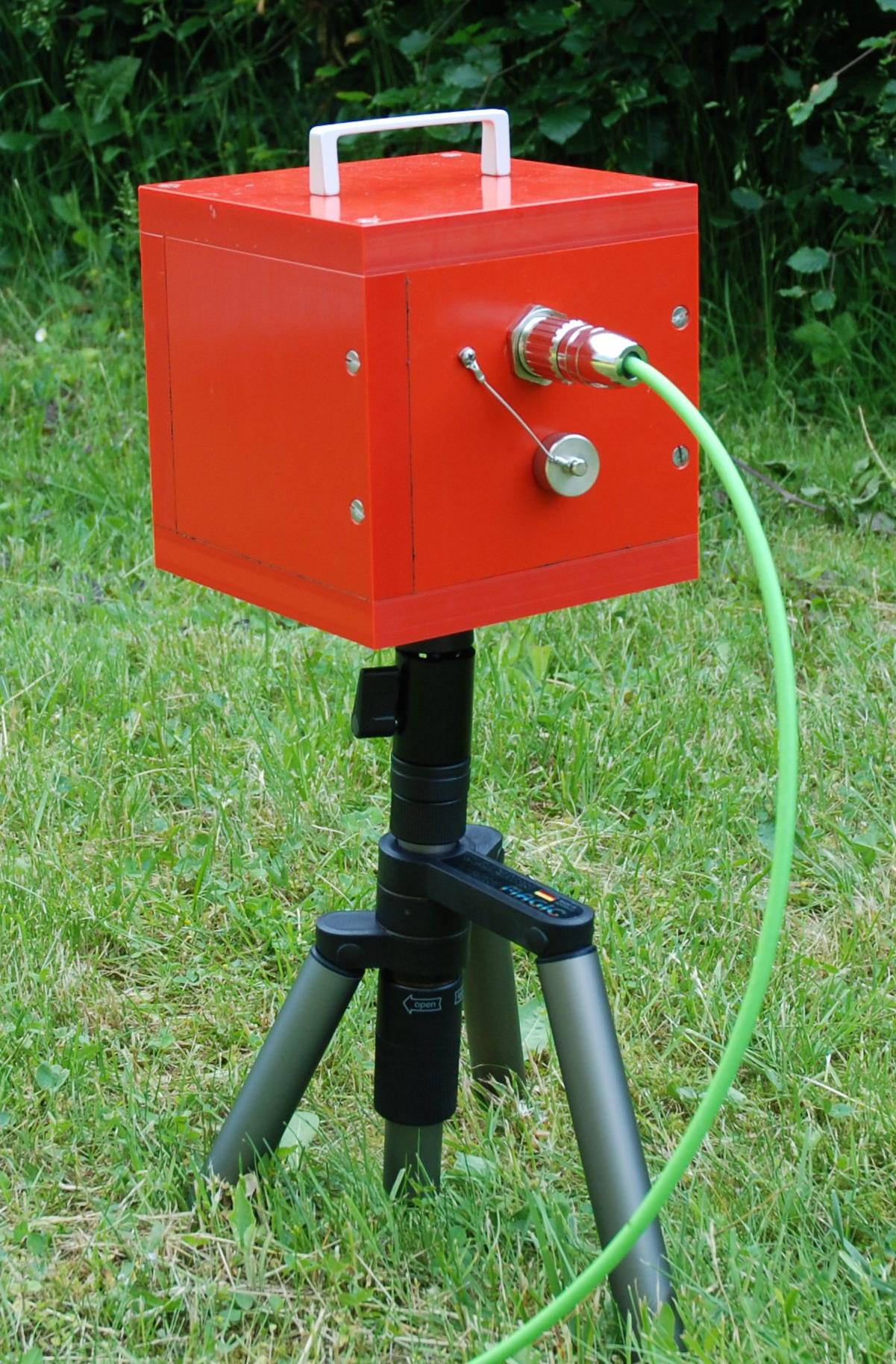
The high-frequency induction coil magnetometer SHFT-02E has been developed to measure variations of the Earth´s magnetic field, particularly for applications in Audio-Magnetotellurics (AMT), Radio Magnetotellurics (RMT) and Controlled Source Magnetotellurics (CSMT, CSEM). It covers a frequency range from 1kHz up to 300 kHz. In spite of its small outer dimensions, the SHFT-02E shows excellent low-noise characteristics. The SHFT-02E is the result of many years of experience of metronix in the design, manufacture and application of induction coil magnetometers.
metronix magnetometers have been used by numerous customers throughout the world - including geophysical exploration companies and research institutes.
Only one SHFT-02E is required to measure the magnetic field in 3 orthogonal axes. The sensors and electronics are enclosed in a shock resistant plastic case that acts as a protection against mechanical stress. The sensor is connected to the metronix ADU-07e data logger (or any other custom electronics) by a cable of up to 10 m length. Special care is taken to the fact that magnetometers are often used under rough environmental influences. The cable has ruggedized water protected push-pull connectors. The high quality of the SHFT-02E data is achieved by a unique design of the ultra-low noise preamplifier.
When connected with an ADU-07e data logger, the sensor type, serial number and transfer function is read out automatically. In this case the user has not to care about transfer function and sensor settings.
Features
The SHFT-02E has several outstanding features which make it a first class instrument for the electromagnetic exploration:
Frequency range from 1 kHz to 300 kHz
3 sensors in one casing
Low noise
Small outline
Wide operating temperature range from -25° C to +60° C
High stability of the sensor´s transfer function
Built-in signal amplification and conditioning electronics
Automatic sensor detection
Automatic transfer of calibration functions
Easy field handling
Technical Data
Frequency range |
1kHz … 300 kHz |
Sensor noise |
\(5 \cdot 10^{- 5} nT/\sqrt{Hz}~@~1000 Hz\) |
\(8 \cdot 10^{- 6} nT/\sqrt{Hz}~@~10000 Hz\) |
|
\(8 \cdot 10^{- 6} nT/\sqrt{Hz}~@~100000 Hz\) |
|
Output sensitivity |
0.05 V/nT f>1000Hz |
for exact values refer to individual calibration file |
|
Output voltage range |
+/- 10V |
Function |
induction coil with current amplifier |
Connector |
30 pole push-pull connector or 10 pole (since 2023, model 8094-0086-00) |
Supply voltage |
+/- 12V to +/-15V stabilized and filtered |
Supply current |
+/- 50mA |
Case |
ruggedized, waterproof case |
Weight |
ca. 5.5 kg |
External dimensions |
l70 mm x 190 mm x 170 mm (L,W,D) |
Operating temperature range |
-25°C … + 60°C |
Sensor
The central part of the SHFT-02E magnetometer are the 3 sensor coils. They consist of a high permeable ferrite core and a few hundred turns of copper wire. Due to its low skin depth the core material prevents the occurrence of eddy currents in the measurement frequency range.
Induction coil sensors do not measure the magnetic field itself but its time derivative. This is expressed in the law of induction:
\(V_{ind} = n \cdot \frac{d\Phi}{dt}\)
with
\(V_{ind}\) |
induction voltage |
\(n\) |
number of turns |
\(\Phi\) |
magnetic flux |
The flux \(\ \Phi\) which flows through one loop of the coil is calculated as
\(\ \Phi = B \cdot A = \mu_{0} \cdot \mu_{c} \cdot H \cdot A\)
with
\(B\) |
magnetic flux density parallel to the sensor axis |
\(\mu_{0}\) |
permeability constant |
\(\mu_{c}\) |
permeability of the core |
\(A\) |
cross section of the core |
\(\overset{\sim}{H}\) |
magnetic field amplitude \((= \hat{H} \cdot e^{j\omega t})\) |
\(f\) |
frequency |
For a sinusoidal magnetic field which can be written with a phasor as \(\overset{\sim}{H} = \hat{H} \cdot e^{j\omega t}\) the induced voltage of the sensor output becomes
\({\overset{\sim}{V}}_{ind} = {\hat{V}}_{ind} \cdot e^{j\omega \cdot t} = j \cdot \underset{S_{0}}{\underbrace{2\pi \cdot n \cdot \mu_{0}\mu_{c} \cdot A}} \cdot f \cdot \hat{H} \cdot e^{j\omega \cdot t} = j \cdot f \cdot S_{0} \cdot \overset{\sim}{H}\)
\(S_{0}\) is defined as the sensor’s sensitivity constant which gives the relation between the magnetic field’s amplitude and the induction voltage. This equation is only a theoretically one. A non ideal sensor’s equivalent circuit does not only contain the field proportional voltage source (which itself is not really proportional) but also some further elements:
Transfer Function of SHFT-02E
The transfer function of the SHFT-02e magnetometer is determined by the transfer function of the preamplifier and the sensor transfer function.
The theoretical overall transfer function is defined by the following equation:
\(F_{Sensor} = \frac{V_{output}}{H} = 0.05\frac{V}{nT} \cdot \frac{P_{1}}{1 + P_{1}}\)
with \(P_{1} = j \cdot \frac{f}{300kHz}\)
This theoretical transfer function is only an approximation of the real transfer function which is obtained by the calibration of the sensor. Each sensor is delivered with a calibration file which has a 3 column ASCII format. The left column represents the frequency, the middle one represents the sensor sensitivity in \(\frac{V}{nT \cdot Hz}\) and the right one the phase in degree.
Calibration by Manufacturer
metronix takes special care of the initial calibration of all SHFT-02E magnetometers as part of the ISO 9001:2015 certified production process. Tests have demonstrated an excellent long time stability of the transfer function.
The calibration is performed in a Helmholtz coil arrangement. It is used to generate a homogeneous magnetic field of known strength as input signal. The input signal for the solenoid coil comes from a frequency response analyzer which is able to perform calculation of transfer functions with a given statistical accuracy.
Each magnetometer is calibrated to a set value of
\(E = 50\frac{mV}{nT}\)
at a frequency of 10 kHz.
A calibration file is generated in a frequency range between 300 Hz and 300 kHz.
Table 4-1 gives an example of a calibration file delivered along with the sensor. Note that not all calibration results are given here due to limited space, gaps are marked by dots.
Each magnetometer is shipped with the original calibration data set which contains the measured values of amplitude and phase of the transfer function over the specified frequency band. Additionally, the calibration data set is stored in an EEPROM chip on the preamplifier and can be read out by the ADU-07e.
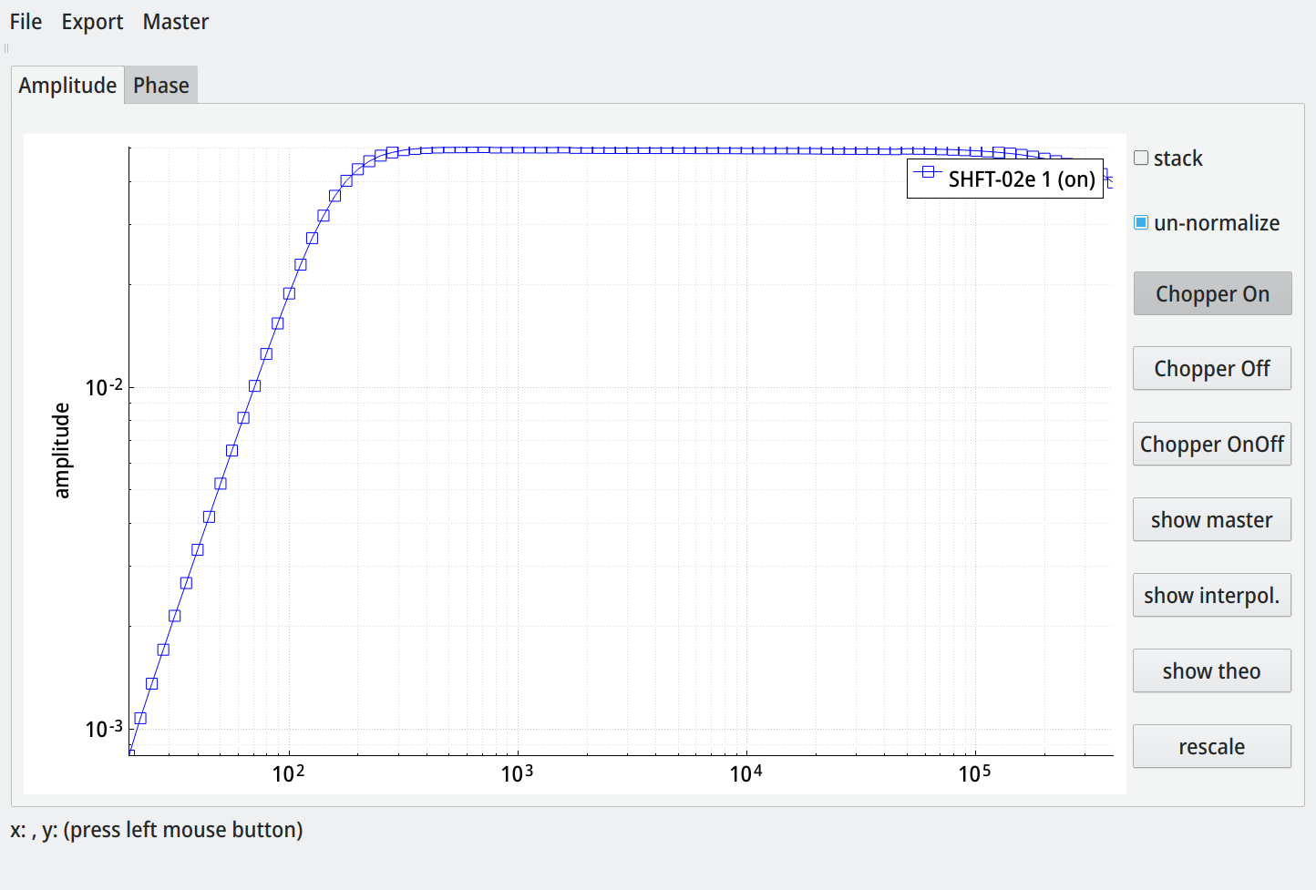
Figure 4-1 and Figure 4-2 show the plots of the calibration function of SHFT-02E (here the x-component).
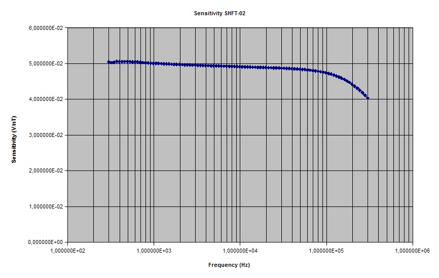
Typical sensitivity calibration curve of SHFT-02E (Ser.#001 x-component)
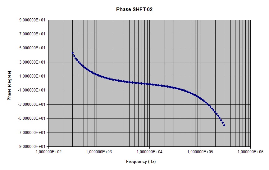
Typical phase calibration curve of SHFT-02E (Ser.#001 x-component)
Mode FRA
Amplitude 1.00E+01
Frequency 1.00E+03
D.C. Offset 0.00E+00
Waveform Sine
Sweep Single
Sweep Start 3.00E+02

SHFT-02E #001 X-Component

Frequency (Hz) Sensitivity V/(nT*Hz) Phase (degrees)

3.000000E+02 1.682466E-04 4.287700E+01
3.216900E+02 1.563255E-04 3.860600E+01
3.449400E+02 1.460239E-04 3.511000E+01
3.698700E+02 1.367787E-04 3.274700E+01
3.966100E+02 1.274981E-04 3.015400E+01
4.252800E+02 1.188892E-04 2.797300E+01
4.560200E+02 1.108112E-04 2.579300E+01
4.889800E+02 1.034252E-04 2.390400E+01
5.243300E+02 9.645234E-05 2.207000E+01
5.622300E+02 8.978493E-05 2.041100E+01
6.028700E+02 8.379996E-05 1.897200E+01
6.464500E+02 7.803376E-05 1.745300E+01
6.931800E+02 7.265600E-05 1.621700E+01
7.432900E+02 6.767203E-05 1.500300E+01
7.970200E+02 6.304465E-05 1.388100E+01
8.546300E+02 5.871369E-05 1.287600E+01
9.164100E+02 5.472398E-05 1.191500E+01
9.826500E+02 5.098221E-05 1.101300E+01
1.053700E+03 4.752811E-05 1.015700E+01
1.129900E+03 4.427693E-05 9.405900E+00
1.211500E+03 4.125191E-05 8.670900E+00
1.299100E+03 3.845253E-05 8.016800E+00
1.393000E+03 3.581924E-05 7.377300E+00
1.493700E+03 3.339674E-05 6.800100E+00
1.601700E+03 3.111260E-05 6.238300E+00
1.717500E+03 2.899484E-05 5.714800E+00
1.841600E+03 2.702229E-05 5.246500E+00
1.974700E+03 2.518642E-05 4.790300E+00
2.117500E+03 2.347167E-05 4.364500E+00
2.270500E+03 2.187741E-05 3.973800E+00
2.434700E+03 2.038788E-05 3.601600E+00
2.610600E+03 1.900541E-05 3.247200E+00
2.799400E+03 1.771342E-05 2.918100E+00
3.001700E+03 1.651012E-05 2.620100E+00
3.218700E+03 1.538994E-05 2.297900E+00
3.451400E+03 1.434406E-05 1.977100E+00
3.700800E+03 1.336971E-05 1.727000E+00
3.968400E+03 1.246385E-05 1.468900E+00
4.255200E+03 1.161576E-05 1.212600E+00
4.562800E+03 1.082645E-05 9.826800E-01
4.892600E+03 1.009434E-05 7.428500E-01
5.246300E+03 9.407286E-06 5.128900E-01
5.625500E+03 8.769127E-06 2.729400E-01
6.032200E+03 8.175075E-06 7.768800E-02
6.468200E+03 7.620510E-06 -1.412200E-0
6.935800E+03 7.103476E-06 -3.592200E-01
7.437100E+03 6.622376E-06 -5.732900E-01
7.974700E+03 6.172387E-06 -7.840200E-01
8.551200E+03 5.754272E-06 -9.971500E-01
9.169300E+03 5.363908E-06 -1.212300E+00
9.832100E+03 5.000014E-06 -1.432800E+00
1.054300E+04 4.656968E-06 -1.656400E+00
1.130500E+04 4.341071E-06 -1.885600E+00
1.212200E+04 4.046627E-06 -2.122200E+00
1.299800E+04 3.772167E-06 -2.365300E+00
1.393800E+04 3.516147E-06 -2.621000E+00
1.494500E+04 3.277718E-06 -2.884800E+00
1.602600E+04 3.055571E-06 -3.154100E+00
1.718400E+04 2.848021E-06 -3.450600E+00
1.842600E+04 2.654828E-06 -3.754500E+00
1.975800E+04 2.474426E-06 -4.072900E+00
2.118700E+04 2.306471E-06 -4.413500E+00
2.271800E+04 2.150044E-06 -4.765100E+00
2.436000E+04 2.003965E-06 -5.142400E+00
2.612100E+04 1.868003E-06 -5.541700E+00
2.800900E+04 1.740483E-06 -5.968500E+00
3.003400E+04 1.622200E-06 -6.421700E+00
3.220500E+04 1.511799E-06 -6.902200E+00
3.453300E+04 1.408910E-06 -7.412800E+00
3.702900E+04 1.313033E-06 -7.961000E+00
3.970600E+04 1.223380E-06 -8.542400E+00
4.257600E+04 1.139994E-06 -9.164000E+00
4.565400E+04 1.062157E-06 -9.828500E+00
4.895400E+04 9.894168E-07 -1.054000E+01
5.249300E+04 9.216501E-07 -1.129900E+01
5.628700E+04 8.584389E-07 -1.211000E+01
6.035600E+04 7.993685E-07 -1.297900E+01
6.471900E+04 7.442789E-07 -1.390000E+01
6.939700E+04 6.927504E-07 -1.489900E+01
7.441300E+04 6.446421E-07 -1.595800E+01
7.979200E+04 5.998023E-07 -1.708700E+01
8.556000E+04 5.578234E-07 -1.829000E+01
9.174500E+04 5.187225E-07 -1.957800E+01
9.837700E+04 4.821408E-07 -2.095500E+01
1.054900E+05 4.479259E-07 -2.242600E+01
1.131100E+05 4.159743E-07 -2.399900E+01
1.212900E+05 3.860046E-07 -2.567400E+01
1.300600E+05 3.579923E-07 -2.746200E+01
1.394600E+05 3.317935E-07 -2.936100E+01
1.495400E+05 3.072275E-07 -3.138200E+01
1.603500E+05 2.842487E-07 -3.353000E+01
1.719400E+05 2.627487E-07 -3.580900E+01
1.843700E+05 2.426204E-07 -3.822300E+01
1.977000E+05 2.237489E-07 -4.077800E+01
2.119900E+05 2.061589E-07 -4.348000E+01
2.273100E+05 1.897575E-07 -4.635000E+01
2.437400E+05 1.744780E-07 -4.940300E+01
2.613600E+05 1.602058E-07 -5.266300E+01
2.802500E+05 1.468324E-07 -5.614700E+01
3.005100E+05 1.343255E-07 -5.982600E+01
Table 4-1: Example for a calibration file of one component
For compatibility the the calibration files may have a “Chopper On” and a “Chopper Off” section. This doesn’t matter; the SHFT does not have a chopper amplifier and the data is exactly the same in both sections.
Sensor Noise
In an electromagnetic measurement system special care has to be taken to noise. The various sources of noise in the system can be summed up to an equivalent input noise voltage at the preamplifier input which is expressed in the equation
\(\sqrt{\frac{\overset{¯}{u^{2}}}{\Delta f}} \approx \sqrt{\frac{\overset{¯}{u_{amp}^{2}}}{\Delta f} + \frac{\overset{¯}{u_{R}^{2}}}{\Delta f} + \frac{\overset{¯}{i_{amp}^{2}}}{\Delta f} \cdot \left( \omega^{2}L^{2} \right)}\)
with
\(\sqrt{\overset{¯}{u_{amp}^{2}}/\mathrm{\Delta}f}\) |
preamplifier noise voltage density (typ. \(0.9nV/\sqrt{Hz}\)) |
\(\sqrt{\overset{¯}{u_{R}^{2}}/\mathrm{\Delta}f}\) |
thermal noise of sensor resistance (typ. \(0.28nV/\sqrt{Hz}\)) |
\(\sqrt{\overset{¯}{i_{amp}^{2}}/\mathrm{\Delta}f}\) |
preamplifier noise current density (typ. \(1pA/\sqrt{Hz}\)) |
In order to reference this noise voltage back to the magnetic field the formula
\(\sqrt{\frac{\overset{¯}{H^{2}}}{\Delta f}} = \frac{\sqrt{\frac{\overset{¯}{u_{}^{2}}}{\Delta f}}}{E_{o} \cdot f} = \frac{1nT}{28.8\mu\;V/\sqrt{Hz} \cdot f} \cdot \sqrt{\frac{\overset{¯}{u_{}^{2}}}{\Delta f}}\)
is used with the sensor coil´s sensitivity of \(E_{0} = 0.02\frac{\mu V}{\sqrt{Hz}}\)
These two equations show that the current noise is spectrally flat whereas the voltage noise of the amplifier and the coil resistance increase proportional with 1/f to low frequencies.
Magnetometer noise is measured at metronix with an HP spectrum analyser. To keep environmental noise away from the sensor the measurements are done with the magnetometer in a multiple shielded chamber.
Figure 5-1 shows the typical noise characteristics of the SHFT-02E.
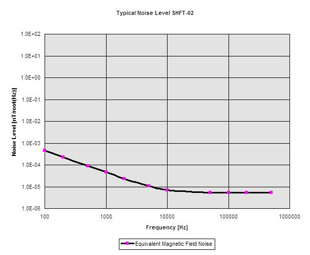
Typical noise curve of SHFT-02E
Installation of Magnetometer
Special care has to be taken to the exact alignment of the magnetometer. The casing of the sensor shows an arrow which must point to the North. The built-in level gives information about the horizontal position of the sensor.
The positive sensor direction points to
X magnetometer to the North
Y magnetometer to the East
Z magnetometer to the ground
A positive flux change in the positive sensor direction will cause a positive change in the output voltage.
Electrical Connection
The metronix magnetometer cables are shielded twisted pair cables which perform optimum protection against external distortion. The connectors have best outdoor characteristics. Nevertheless, care should be taken to avoid intrusion of particles. Each connector has a protection cap which can be removed by pulling. Please ensure that the expensive connectors are always protected by the caps during assembling or disassembling of the MT system.
To connect a cable to a magnetometer rotate it to the red coded position, put connector into the input plug and just push until it snaps in.
The SHFT-02E can be directly connected to the ADU-07e data logger. Use the multi-purpose connector Input 2 to connect the sensor with the ADU-07e.
In case that other custom electronics are used a connection should be simple according to the pin assignment given in
Table 7-1.
Caution
Special care must be taken with custom electronics to avoid a wrong use of the power supply inputs! The magnetometer electronics may be damaged immediately if the power is connected the wrong way!
Pinout of External Connectors
The following tables show the wiring of the connectors of the SHFT-02E, old version until 2023 (8094-0082-00)
Pinout of SHFT-02E socket
Socket (SHFT-02E socket) |
Signal |
Category |
|---|---|---|
1 |
+12V |
Power |
2 |
-12V |
Power |
3 |
SGND |
Screen |
4 |
SGND |
Screen |
5 |
n.c. |
|
6 |
n.c. |
|
7 |
n.c. |
|
8 |
n.c. |
|
9 |
Hx Signal |
Signal |
10 |
Hx GND |
Signal |
11 |
Hy Signal |
Signal |
12 |
HY GND |
Signal |
13 |
Hz Signal |
Signal |
14 |
HZ GND |
Signal |
15 |
n.c. |
|
16 |
n.c. |
|
17 |
n.c. |
|
18 |
n.c. |
|
19 |
n.c. |
|
20 |
n.c. |
|
21 |
n.c. |
|
22 |
n.c. |
|
23 |
n.c. |
|
24 |
n.c. |
|
25 |
\(I^{2}C\) SDATA |
Logic |
26 |
\(I^{2}C\) SDATA |
Logic |
27 |
n.c. |
|
28 |
n.c. |
|
29 |
n.c. |
|
30 |
n.c. |
Pin-out of magnetometer cable
Origin ODU MiniSnap Series K, 30 pole S23K0N-P30PFG0-0200 |
Origin ODU MiniSnap Series K, 30 pole S23K0N-P30PFG0-0200 |
Signal |
Colour |
Cat. |
|---|---|---|---|---|
1 |
1 |
+12V |
white |
twist w. 9 |
2 |
2 |
-12V |
black |
twist w.10 |
3,4 |
3,4 |
Screen |
||
9 |
9 |
HX Signal |
green |
\ twist |
10 |
10 |
HX GND |
yellow |
/ ed |
11 |
11 |
HY Signal |
grey |
\ twist |
12 |
12 |
HYGND |
pink |
/ ed |
13 |
13 |
HZ Signal |
blue |
\ twist |
14 |
14 |
HZ GND |
red |
/ ed |
25 |
25 |
SDATA |
brown |
twist w. 1 |
26 |
26 |
SCLK |
violet |
twist w. 2 |
For the newer SHFT-02E (8094-0086-00) the pinout is here :ref:multi_purpose_con
Trouble Shooting
This chapter describes our experience to localise possible errors of the system and methods how to fix them or get around it.
Check of Magnetometer Cable
The pin-out of the magnetometer cable is given in chapter 7. Check the cable by using an Ohm-meter pin by pin according to the table. Also check for damages of the cable´s isolation.
Parallel Sensor Test
In case you own two or more SHFT-02E sensors you could perform a parallel sensor test. You should position the sensors side by side with a distance of 2 m and both pointing to the North. Start a short recording and compare the signals of the 3 components.
Extended Calibration
An extended calibration down to 20 Hz can be done on request.
This is for CSEM and airborne with active sources (transmitter) only. Natural signals can not be recorded for f < 300 Hz.
Additionally the ADU-08e switches a 500 Hz high pass filter when recording 8 kHz and higher. CSEM jobs for lower frequencies must be configured
Environmental
In case the item is no longer needed, please dispose it according to the local regulations for electronic waste.
Dispose items only at qualified places, not in your household waste.

WEEE Reg. DE 25690185