MFS-10e
Product Description
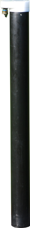
The broadband induction coil magnetometer MFS-10e has been developed to measure variations of the Earth´s magnetic field, particularly for applications in Magnetotellurics (MT). It is mainly intended for use as a vertical sensor. The connector shows downward and the size of the coil is 29 cm shorter than the MFS-06e sensor. A wide frequency range from 0.0001 Hz up to 10 kHz is covered, best range up to 1 kHz (due to the shorter length and much more windings the noise level above 1 kHz is higher compared to the MFS-06e). In spite of its broad bandwidth, the MFS-10e shows very good low-noise characteristics, extremely low temperature drift of input offset voltage and offset current and a very stable transfer function over temperature and time. The MFS-10e is the result of many years of experience of metronix in the design, manufacture and application of induction coil magnetometers. As a unique feature the MFS-10e acts as an “intelligent plug and play” sensor. Thus, once connected to the ADU-07e, it will send its type and serial number as well as its calibration function to the ADU-07e automatically. The user does not have to care about any further sensor parameter setup.
metronix magnetometers have been used by numerous customers all over the world - including geophysical exploration companies and research institutes.
The sensor is enclosed in a shock resistant cylindrical tube that acts as a protection against mechanical stress. The tube is waterproof and also resistant to ultraviolet radiation. The magnetometer contains the electronics for pre-amplification of the sensor signal as well as for precise self calibration. The MFS-10e magnetometer is connected to the metronix ADU-07e data logger (or any other custom electronics) by a cable of up to 70 m in length. Special care is taken to the fact that magnetometers are often used under rough environmental influences. All cables have ruggedized waterproof connectors. The high quality of the MFS-10e data is achieved by a unique design for the ultra low noise and low frequency preamplifier.
Features
The MFS-10e has several outstanding features which make it a first class instrument for the electromagnetic exploration:
Wide frequency range from 1/10000 Hz to 1 kHz (10 kHz)covered by only one sensor
High linearity
Low noise
High accuracy calibration with built-in precision calibration facility
Wide operating temperature range from -25° C to +60° C
High stability of the sensor´s transfer function due to magnetic field feedback
Built-in signal amplification and conditioning electronics
Metronix “Smart Sensor” technology – sensor parameters incl. transfer function can be read by ADU-07e automatically
Especially suited for measurement of the vertical magnetic field.
29cm shorter than MFS-06e
Technical Data
Frequency range |
0.0001 Hz ….. 1 kHz (10 kHz) |
Frequency bands |
0.0001 Hz ….. 500 Hz (chopper on) |
10 Hz ….10 kHz (chopper off) |
|
Sensor noise |
\(1.5 \cdot 10^{- 2} nT/\sqrt{Hz}~@~0.01 Hz\) |
\(1.5 \cdot 10^{- 4} nT/\sqrt{Hz}~@~1 Hz\) |
|
\(3.5 \cdot 10^{- 6} nT/\sqrt{Hz}~@~1000 Hz\) (chopper off) |
|
Output sensitivity |
0.2 V/(nT*Hz) f<< 4Hz |
0.8 V/nT f>> 4Hz |
|
for exact values refer to individual calibration file |
|
Output voltage range |
+/- 10V |
Function |
induction coil with magnetic field feed back |
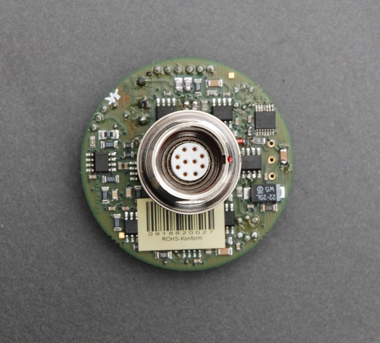
Connector |
10 pole ODU Series K |
Calibration coil sensitivity |
4 nT / V |
Feedback cut-off frequency |
4 Hz |
Supply voltage |
+/- 12V to +/-15V stabilised and filtered |
Supply current |
+/- 25mA |
Case |
ruggedized, waterproof plastic case |
Weight |
ca. 9 kg |
External dimensions |
length 860 mm, diameter 75mm |
Operating temperature range |
-25°C ….. + 60°C |
Sensor
The central part of the MFS-10e magnetometer is the sensor coil. It consists of a high permeable ferrite core and several thousand turns of copper wire. Due to its low skin depth the core material prevents the occurrence of eddy currents in the measurement frequency range.
To achieve good mechanical stability the main structure of the sensor is based on the cylindrical tube which is made of fibre glass reinforced epoxy.
Induction coil sensors do not measure the magnetic field itself but its time derivative. This is expressed in the law of induction:
\(V_{ind} = n \cdot \frac{d\Phi}{dt}\)
with
\(V_{ind}\) |
induction voltage |
\(n\) |
number of turns |
\(\Phi\) |
magnetic flux |
The flux \(\ \Phi\) which flows through one loop of the coil is calculated as
\(\ \Phi = B \cdot A = \mu_{0} \cdot \mu_{c} \cdot H \cdot A\)
with
\(B\) |
magnetic flux density parallel to the sensor axis |
\(\mu_{0}\) |
permeability constant |
\(\mu_{c}\) |
permeability of the core |
\(A\) |
cross section of the core |
\(\overset{\sim}{H}\) |
magnetic field amplitude \((= \hat{H} \cdot e^{j\omega t})\) |
\(f\) |
frequency |
For a sinusoidal magnetic field which can be written with a phasor as \(\overset{\sim}{H} = \hat{H} \cdot e^{j\omega t}\) the induced voltage of the sensor output becomes
\({\overset{\sim}{V}}_{ind} = {\hat{V}}_{ind} \cdot e^{j\omega \cdot t} = j \cdot \underset{S_{0}}{\underbrace{2\pi \cdot n \cdot \mu_{0}\mu_{c} \cdot A}} \cdot f \cdot \hat{H} \cdot e^{j\omega \cdot t} = j \cdot f \cdot S_{0} \cdot \overset{\sim}{H}\)
\(S_{0}\) is defined as the sensor’s sensitivity constant which gives the relation between the magnetic field’s amplitude and the induction voltage. This equation is only a theoretically one. A non ideal sensor’s equivalent circuit does not only contain the field proportional voltage source (which itself is not really proportional) but also some further elements:
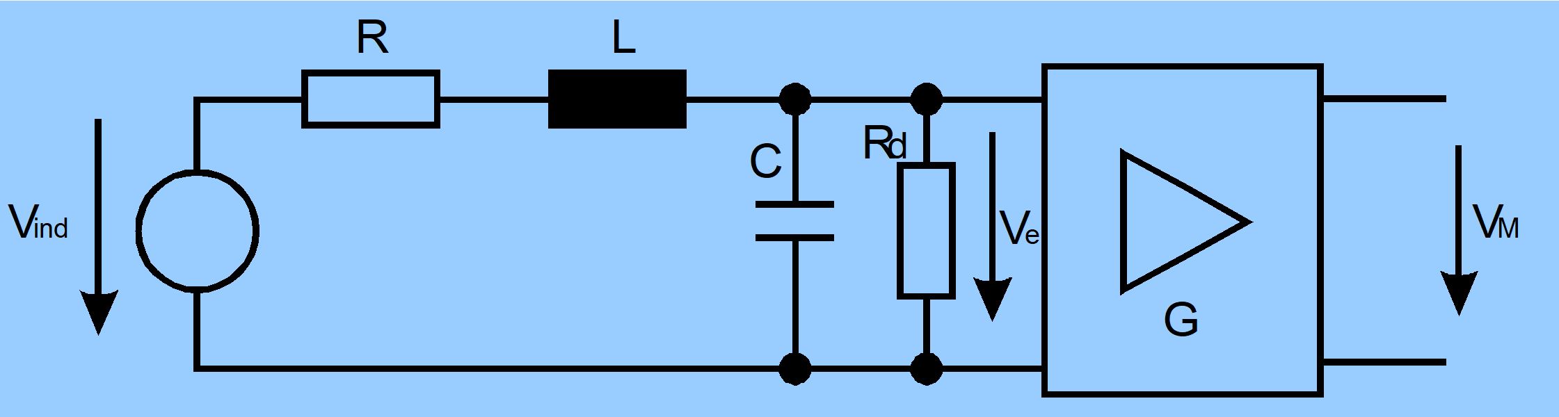
Simplified equivalent circuit diagram for a sensor coil
Referring to the source, the induced sensor voltage \(V_{ind}\), the coil resistance \(R\), the input resistance of the amplifier \(R_{d}\) the coil inductivity \(L\) and the capacity \(C\) yield a damped serial resonance circuitry. The transfer function of the sensor will show a strong peak at its resonance frequency.
For the sensor itself, without the preamplifier, we get the transfer function
\(\frac{V_{e}}{V_{ind}} = \frac{\left. {R_{d}/\left( R_{d} + R \right.} \right)}{1 - \left( f/f_{0})^{2} + j \cdot 2D \cdot \left( f/f_{0} \right) \right.}\)
with the amplifier’s input resistance \(R_{d}\), Gain \(G\), resonance frequency \(f_{0}\) and attenuation \(D\) defined as
\(f_{0} = \frac{1}{2\pi \cdot \sqrt{a \cdot L \cdot C}}\) \(~a = \frac{R_{d}}{R + R_{d}}\) \(G = \frac{V_{M}}{V_{e}}\) \(2D = \sqrt{\frac{R_{d}}{R_{d} + R}} \cdot \frac{\sqrt{L/C}}{R_{d}} + \frac{R}{\sqrt{L/C}}\)
Having this in mind the resulting transfer function between the magnetic field and the sensor output voltage becomes
\(F_{sensor} = \frac{\hspace{0pt}\hspace{0pt}\hspace{0pt}V_{e}}{\overset{\sim}{H}} = \frac{j \cdot S_{0} \cdot {R_{d}/\left( R_{d} + R \right)} \cdot f}{1 - \left( f/f_{0})^{2} + j \cdot 2D \cdot \left( f/f_{0} \right) \right.}\)
The equivalent circuit diagram of the magnetometer leads to a frequency dependent sensitivity \(E(f)\) referred to the preamplifier output of:
\(E\left( f \right) = E_{0} \cdot \frac{V_{e}}{V_{ind}}\)
with
\(E_{0} = G \cdot S_{0}\)
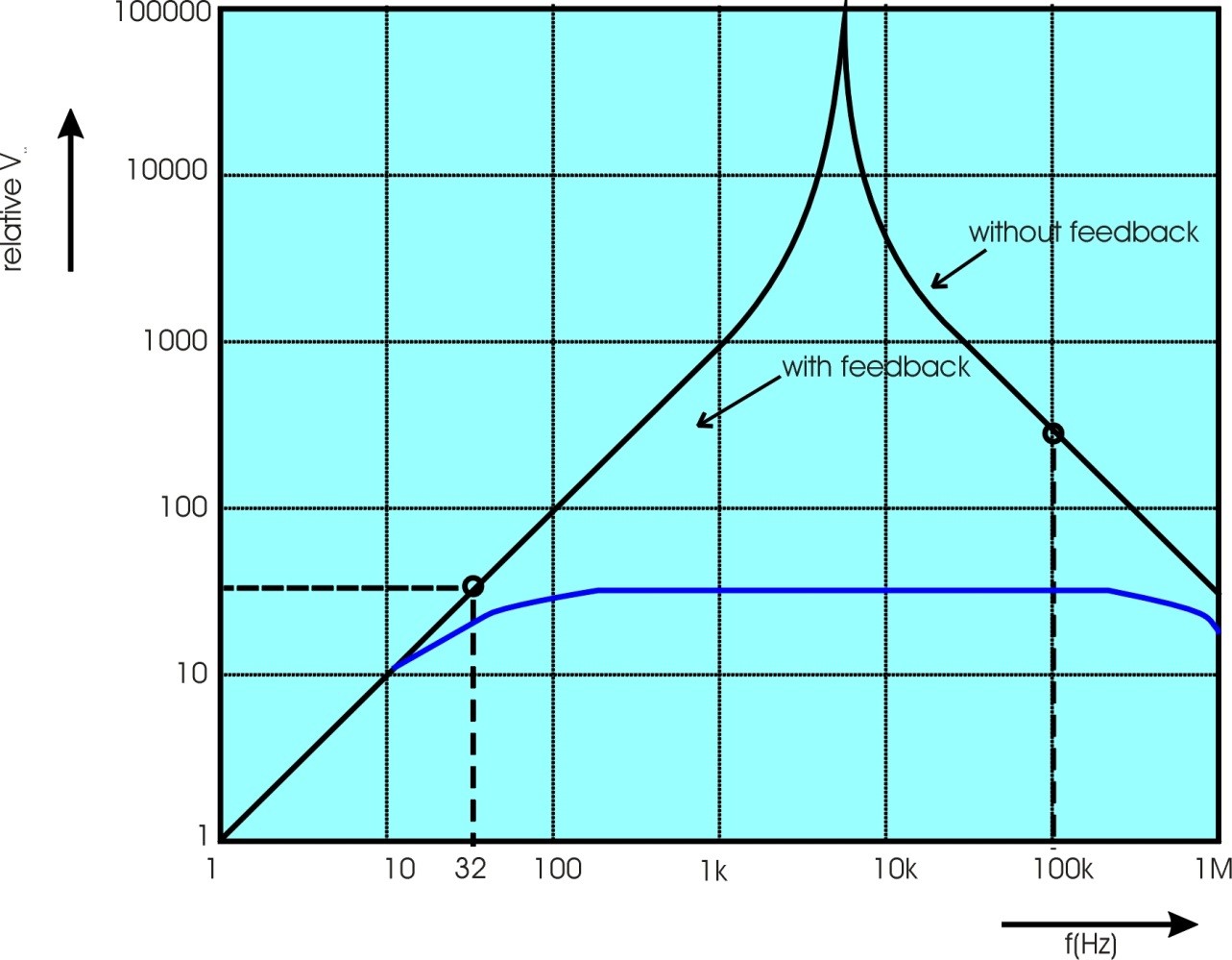
Relative frequency response of magnetometer MFS-10e for \(H(f) = const\).
Figure 2-2 shows the principle frequency response of the output voltage \(V_{m}\) of the MFS-10e. Considering the feedback, the output voltage is given by:
\(V_{M}\left( f \right) = \frac{j \cdot f \cdot H\left( f \right) \cdot E\left( f \right)}{1 + j\frac{f}{f_{c}}}\)
The cut-off frequency of the magnetometer is set to \(f_{c} = 4Hz\).
Please consider that this figure shall only explain the feedback principle. Additional effects caused by the low-pass filtering of the sensor signal at \(8192 Hz\) and other influences are not respected here.
Preamplifier
The integrated preamplifier performs the signal amplification of the sensor output voltage as well as the conditioning of the magnetic field feedback signal and allows to feed-in an external calibration signal. Special care has been taken to avoid disturbance of the electronics by external electromagnetic noise.
To achieve DC characteristics close to the physical limits, the preamplification electronics is split into a lower frequency path (low-pass corner frequency \(330 Hz\)) which is chopper stabilized in order to achieve excellent low-noise and drift characteristics and a separate AC path with the same corner frequency. The output signals of these two amplification paths are used as an input for the magnetic feedback conditioning stage.
The following block diagram explains the design:
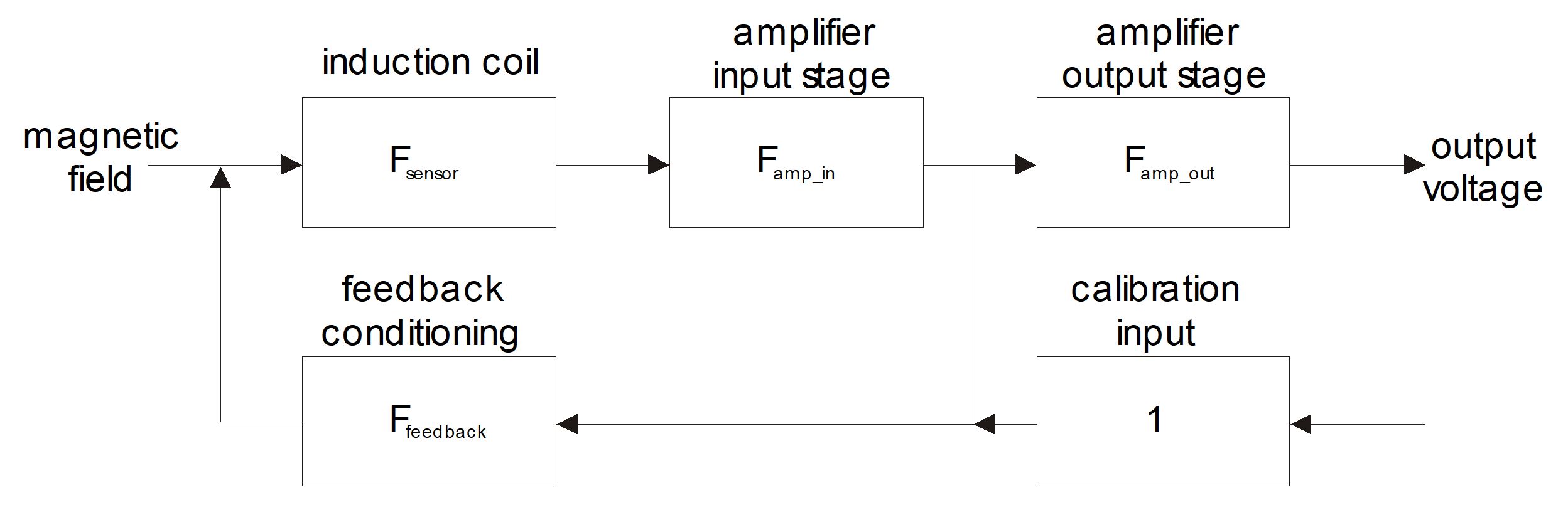
MFS-10e block diagram
The resulting frequency characteristics of the MFS-10e sensor system is dominated by the feedback loop. As it was demonstrated in chapter 2 of this manual, the characteristics of the sensor itself mostly depends on the resonance circuit formed by the main impedance and main capacity of the coil. This leads to a strong peek in the spectrum at the resonance frequency \(f_{0}\).
In the block diagram above the summing function for the input node leads to the transfer function, assuming that \(U_{pre}\) is the output voltage of the amplifier input stage:
\(\left( H - U_{pre} \cdot F_{FB} \right) \cdot F_{sensor} \cdot F_{amp\_ in} = U_{pre}\)
which is the same as
\(\frac{U_{pre}}{H} = \frac{1}{\left( F_{sensor} \cdot F_{amp\_ in} \right)^{- 1} + F_{FB}}\)
Close to the resonance frequency the influence of the sensor transfer function disappears and the overall characteristics depends mainly on \(F_{FB}\). This results in a flat frequency response of the sensor system over the whole frequency band of interest.
Additionally the preamplifier electronics contains an output line driver which provides an \(8 kHz\) low-pass filter. The output buffer is able to drive cables up to 70 m length.
Preamplifier of MFS-10e
Transfer Function of MFS-10e
The transfer function of the MFS-10e magnetometer is determined by the transfer function of the preamplifier, the feedback electronics and the sensor transfer function.
The theoretical overall transfer function is defined by the following equations:
\(F_{Sensor} = \frac{V_{output}}{H} = 0.8\frac{V}{nT} \cdot \frac{P_{1}}{1 + P_{1}} \cdot \frac{1}{1 + P_{2}}\)
with
\(P_{1} = j \cdot \frac{f}{4Hz}\) \(P_{2} = j \cdot \frac{f}{8192Hz}\)
This theoretical transfer function is only an approximation of the real transfer function (approx. up to \(500 Hz\) with Chopper On) which is delivered by the calibration of the sensor. Each sensor is delivered with a calibration file which has a 3 column ASCII format. The left column represents the frequency, the middle one represents the sensor sensitivity in \(\frac{V}{nT \cdot Hz}\) and the right one the phase in degree.
As it can be easily calculated from the equation above, for very low frequencies the transfer function of the coil converges to \(\frac{0.2V}{nT \cdot Hz}\) in amplitude and to 90 degrees in phase. The calibration data which is delivered along with the coil ends at its low end at \(f = 0.1 Hz\). The amplitude can be taken as the given value at \(0.1 Hz\) also for lower frequencies. The phase value for very low frequencies \(<0.1Hz\) can be computed to
\(\varphi = atan\left( \frac{4Hz}{f} \right)\) with \(f < 0.1Hz\)
In addation to the delivered calibration file the sensor is equipped with the calibration data stored on a chip inside the sensor. This information will be read by the ADU-07e. Each time a data recording is done this calibration data is stored along with the recording data.
Integrated Calibration Facility
The integrated calibration facility makes it easy for the user to perform an online calibration or test of the magnetometer transfer function. A differential test signal can simply be injected into the inputs and is internally added to \(U_{pre}\) without further amplification as shown in Figure 3-1. A voltage on the input results in a magnetic field according to
\(H = 4\frac{nT}{V} \cdot U_{cal}\)
This makes it easy to calculate the resulting transfer function of the magnetometer using the formula
\(F_{MFS - 06} = \frac{U_{out}}{U_{cal}} \cdot \frac{1}{4\frac{nT}{V} \cdot f}\)
External magnetic field variations do not disturb the measurement if a correlation analyser (e.g. Solartron 1250) is used. The max. allowed signal amplitude on the calibration input is \(\pm 10V\) but it has to be considered that the sensor may be saturated at higher frequencies. For example at \(10 Hz < f < 10kHz\). The maximum amplitude shoud not exceed \(80mV\).
If the metronix ADU-07e is used as data logger the magnetometer characteristics will be tested regularly as a part of the normal system self test.
Calibration by Manufacturer
metronix takes special care of the initial calibration of all MFS-10e magnetometers as part of the ISO 9001:2015 certified production process. Tests have demonstrated an excellent long time stability of the transfer function.
The calibration is performed in the „Magnetsrode“ geomagnetic laboratory which is operated by the Institute of Geophysics at the Technical University of Braunschweig, mostly to calibrate space flight magnetometers. It offers special environmental circumstances and has an extremely low distortion level.
A large solenoid (l = 3.6 m; d = 30 cm) has been calibrated by a reference sensor with an accuracy of better than ±0.2%. It is used to generate a homogeneous magnetic field of known strength as input signal. The input signal for the solenoid comes from a N4L PSM3750 phase sensitive multimeter which is able to perform calculation of transfer functions with a given statistical accuracy.
Each magnetometer is calibrated to a sensitivity
\(E = 0.2\frac{V}{nT \cdot Hz}\)
at a frequency of 0.1 Hz.
A calibration file is generated in a frequency range between 0.1 Hz and 10 kHz. Lower frequency calibration is not required because the sensor obeys the mathematical rules (theoretical transfer function with a very high precision.
  Calibration measurement with NumetriQ PSM 3750 - 0.1.100000.1.33

Metronix GmbH, Kocherstr. 3, 38120 Braunschweig
Magnetometer: MFS10e#023 Date: 15/10/28 Time: 08:47:03
FREQUENCY MAGNITUDE PHASE

Hz V/(nT\*Hz) deg

Chopper On
+1.0000E-01 +1.9942E-01 +8.8596E+01
+1.2328E-01 +1.9955E-01 +8.8248E+01
+1.5199E-01 +1.9959E-01 +8.7817E+01
+1.8738E-01 +1.9927E-01 +8.7355E+01
+4.3287E-01 +1.9855E-01 +8.3939E+01
. . .
. . .

+5.3367E+03 +1.5014E-04 -3.6649E+01
+6.5793E+03 +1.1454E-04 -5.0802E+01
+8.1113E+03 +8.5612E-05 -6.3095E+01
+1.0000E+04 +6.1500E-05 -7.6150E+01

Chopper Off
+1.0000E+00 +1.8611E-01 +1.1322E+02
+1.2329E+00 +1.9701E-01 +1.0381E+02
+1.5199E+00 +2.0259E-01 +9.4129E+01
+1.8738E+00 +2.0258E-01 +8.4332E+01
. . .
. . .
+4.3288E+03 +1.5478E-04 -2.7471E+01
+5.3367E+03 +1.5047E-04 -3.6406E+01
+6.5793E+03 +1.1493E-04 -5.0515E+01
+8.1113E+03 +8.5958E-05 -6.2768E+01
+1.0000E+04 +6.1826E-05 -7.5739E+01
Table 6-1 gives an example of a calibration file delivered along with the sensor. Note that not all calibration results are given here due to limited space, gaps are marked by dots here.
Each magnetometer is shipped with the original calibration data set which contains the measured values of amplitude and phase of the transfer function over the specified frequency band.
The calibration file is split into 2 sections. The first section shows the results with the chopper switched on (LF mode) whilst the second section shows the results with the chopper amplifier switched off (HF mode).
Figure 6-1 and Figure 6-2 show the plots of the calibration function of MFS-10e Ser. #002.

Typical sensitivity calibration curve of MFS-10e (here Ser.#001)
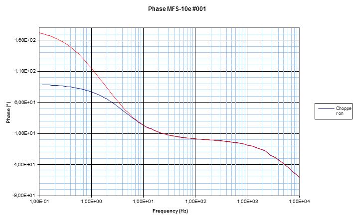
Typical phase calibration curve of MFS-10e (here Ser.#001)
Sensor Noise
In an electromagnetic measurement system special care has to be taken to noise. The various sources of noise in the system can be referenced back to an equivalent input noise voltage at the preamplifier input for comparison purpose which is expressed in the equation
\(\sqrt{\frac{\overset{¯}{u^{2}}}{\Delta f}} \approx \sqrt{\frac{\overset{¯}{u_{amp}^{2}}}{\Delta f} + \frac{\overset{¯}{u_{R}^{2}}}{\Delta f} + \frac{\overset{¯}{i_{amp}^{2}}}{\Delta f} \cdot \left( \omega^{2}L^{2} \right)}\)
with
\(\sqrt{\overset{¯}{u_{amp}^{2}}/\mathrm{\Delta}f}\) |
preamplifier noise voltage density (typ. \(1.9nV/\sqrt{Hz}\)) |
\(\sqrt{\overset{¯}{u_{R}^{2}}/\mathrm{\Delta}f}\) |
thermal noise of sensor resistance (typ. \(3.8nV/\sqrt{Hz}\)) |
\(\sqrt{\overset{¯}{i_{amp}^{2}}/\mathrm{\Delta}f}\) |
preamplifier noise current density (typ. \(10fA/\sqrt{Hz}\)) @chopper off |
To reference this noise voltage back to the magnetic field the formula
\(\sqrt{\frac{\overset{¯}{H^{2}}}{\Delta f}} = \frac{\sqrt{\frac{\overset{¯}{u_{}^{2}}}{\Delta f}}}{E_{o} \cdot f} = \frac{1nT}{30\mu\;V/\sqrt{Hz} \cdot f} \cdot \sqrt{\frac{\overset{¯}{u_{}^{2}}}{\Delta f}}\)
is used. These two equations show that the current noise is spectrally flat whereas the voltage noise of the amplifier and the coil resistance increase proportional with 1/f to low frequencies. For higher frequencies it is possible to eliminate a part of the preamplifier noise if the chopper path is switched off. This can be done with a pulse on the HCHOP line.
The noise of the magnetometer is measured by a parallel sensor test. The correlation between two parallel located sensors is determined and by this means, in connection with the measured amplitude spectra, the noise of the sensor can be computed.
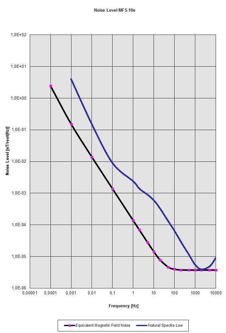
Typical Noise Chart of the MFS-10e in comparison with the natural magnetic field varitions on a quiet day
Installation of Magnetometers
To avoid low frequency distortion due to mechanical vibrations of the sensor it must be dug into the soil. If this is not done, significant noise caused by wind may be created which can make a measurement unusable. The z component magnetometer should be dug into the soil at least to the amount of half of its size. In order to obtain optimum results the free end of the sensor should be covered by a protection cap like a plastic bucket.
Special care must be taken to the exact alignment of the magnetometer tube. It’s bottom side (that one without the cable connector) must point exactly to the corresponding (positive sensor) direction:
MFS-06e \(H_{X}\) magnetometer to the North
MFS-06e \(H_{Y}\) magnetometer to the EAST
MFS-06e \(H_{Z}\) magnetometer to the ground
A positive flux change in the positive sensor direction will cause a positive change in the output voltage.
Electrical Connection
All magnetometer cables from metronix are shielded twisted pair cables which perform optimum protection against external distortion. Connectors have best outdoor characteristics including water tightness. Nevertheless, care should be taken to avoid intrusion of particles. Each connector has a protection cap which can be removed by just pulling it off. Please ensure that the expensive connectors are always protected by the caps during assembling or disassembling of the MT system.
To connect a cable to a magnetometer rotate it to the coded position (red dot to red dot), put connector into the input plug and lock it by pushing it until it snaps in.
The MFS-10e can be directly connected to the ADU-07e data logger. Due to the easy setup procedure of a metronix GMS-07 system, the magnetometer cables simply have to be put into the corresponding ADU-07 ports.
In case other custom electronics is used the production of a suitable cable connection should not be too difficult according to the pin assignment given below.
Caution
Special care must be taken with custom electronics to avoid a wrong use of the power supply inputs! The magnetometer electronics may be damaged immediately if the power is connected the wrong way!
Note
The Chopper On/Off Signal is a standard CMOS input. Low level (<0.5V) will switch the chopper amplifier off. High level (>3.5V up to 13V) will switch the chopper on. If you use the sensor with custom electronics, make sure to switch the chopper line on and off with a delay of about 100ms or more in order to properly initialize the sensor.
Installation with ADU-07e
This chapter describes the setup of the MFS-10e in the field in connection with the ADU-07e.
Standard 5-channel MT Setup
Figure 8-1 illustrates the field setup of a five channel MT station. Only a few components are required:
ADU-07e with battery and GPS antenna
3 magnetometers like MFS-06e, MFS-07e, MFS-10e.(MFS-10e is used as vertical sensor)
3 magnetometer cables
4 electric field probes
4 electric field cables
1 grounding rod + cable
Field computer (temporarily - may be any ruggedized laptop)
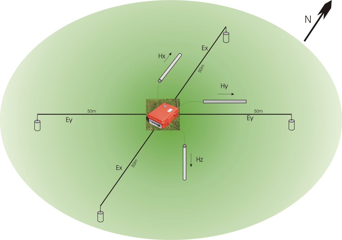
Typical 5-channel MT field setup
Connection of the Sensors to the ADU-07e
Now you can install the sensors:
Dig the four EFP-06 into the soil and connect them with the input of the E-Field cable drum.
Connect the other end of the 50m E-cable with the appropriate input terminals of the ADU-07e. The North-probe will be connected with the terminal labelled “N” of the ADU-07e. In the same way the “S”, “E”, “W” input terminals of the ADB are connected with the corresponding probes. Make sure that the E-Field cables are unreeled completely and the cable is not moving in the wind.
Stick-in the delivered grounding rod close to the ADU-07e and connect it with the black GND-input clamp of the ADU-07e.
Connect one end of the magnetometer cables with the HX, HY resp. HZ magnetometer. For this purpose first remove the magnetometer’s protection cap. Now push the end of the cable through the rubber flap in the middle of the protection cap. After having it connected with the socket properly, the magnetometer’s protection cap is pushed over the magnetometer’s head again. Please note that the reel of the magnetometer cable (if there is one) always should be placed near the ADU-07e. The exact positioning and installation procedure of the magnetometer is described below. It is very important to notice the hints given there in order to obtain best results.
Connect the plugs on the other end of the magnetometer cables with the corresponding input sockets on the ADU-07e i.e. the cable of the HX sensor with the socket labelled “HX”, the cable of the HY sensor with the “HY” socket and the cable of the HZ sensor with the “HZ” socket of the ADU-07e.
The correct direction of the sensors can be fixed by using a compass and two sticks:
A field helper rams the first stick into the soil according to the command of the other helper with the compass. The second stick is rammed behind the first stick. The correct alignment is found when the needle of the compass points to North for HX resp. East for HY and the sticks as well as the ring and bead sights of the compass are in line.
The horizontal direction is balanced using a level. The exact vertical position of the HZ-magnetometer can also be fixed by a level.
The magnetometers must be installed in a way that any movement of the sensors due to micro-vibrations is avoided. Such motion of an induction coil magnetometer in the stationary earth magnetic field would cause significant artificial noise. For this reason the horizontal magnetometers must be dug and covered by soil completely. The vertical HZ-component should be dug-in to at least half of its length or better to 4/5 of its length. An additional coverage of the HZ sensor by a plastic bucket helps to reduce wind influences.
Note
The cables close to the magnetometers must be fixed in a way that they cannot move in the wind!!
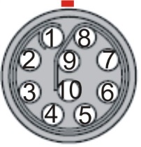
Pinout of Connector Socket
Socket 10-pole ODU MiniSnap G32K0C-P10QJ00-0000 Pin |
Signal |
1 |
+12V |
2 |
-12V |
3 |
H-Chop |
4 |
Sensor GND |
5 |
Cal Signal+ |
6 |
Cal Signal - |
7 |
Input + |
8 |
Input - |
9 |
\(I^{2}C\) SDA |
10 |
\(I^{2}C\) SCL |
The picture below shows the front side of the socket or the rear side of the corresponding plug with the solder cups.
You can order a suitable cable plug from Metronix or directly from the manufacturer ODU in Germany(www.odu.de <http://www.odu.de>)
The part number of the plug is ODU Minisnap Series K S22K0C-P10MJG0-700S
You may also need a strain relief streeve ODU part.no. 702023205965060
Target ODU MiniSnap Series K 10 pole |
Origin ODU MiniSnap Series K 10 pole |
Signal |
Colour |
Cat. |
1 |
1 |
+12V |
white |
\ twist |
9 |
9 |
SDATA |
brown |
/ ed |
3 |
3 |
HCHOP |
green |
\ twist |
4 |
4 |
GND |
yellow |
/ ed |
5 |
5 |
+CAL |
grey |
\ twist |
6 |
6 |
-CAL |
pink |
/ ed |
7 |
7 |
Signal out |
blue |
\ twist |
8 |
8 |
Signal Return |
red |
/ ed |
2 |
2 |
-12V |
black |
\ twist |
10 |
10 |
SCLK |
violet |
/ ed |
Case |
Case |
Screen |
Trouble Shooting
This chapter describes our experience to localise possible errors of the system and methods how to fix them or get around it.
Parallel Sensor Test
In order to check the functionality of the sensors it is a good idea to perform a so called parallel sensor test. For this purpose 2 or more magnetometers are positioned horizontally and parallel with a distance of about 2 m from each other. Dig in the magnetometers. The electric field lines are laid out in parallel and perpendicular to the magnetic sensors. Use a single probe for each line (all together four of them). Now you record time series. If everything works fine you must see well correlated time series of the electric and the magnetic channels. A noisy sensor can be found out by this method easily.
Check of Magnetometer Cable
The pin-out of the magnetometer cable is given in chapter 0. Check the cable by using an Ohm-meter pin by pin according to the table. Also check for damages of the cable´s isolation.
Caution
Never pull the sensor out of the soil on its cable because either the cable connector or the sensor socket will be damaged by this procedure.
In Situ Measurement of Transfer Function
Metronix provides a software tool which allows to check the sensor´s transfer function in the field. This is achieved by a special joblist running on the ADU-07e which records some data for about half an hour. In course of this procedure test signals are fed into the calibration coil of the magnetometer. The software reads and processes the data and delivers the transfer function of the sensor as a result. You will find the necessary software on the USB key delivered along with the ADU-07e (subfolder software). MFS-10e is tested with the MFS-06e joblist.
Environmental
In case the item is no longer needed, please dispose it according to the local regulations for electronic waste.
Dispose items only at qualified places, not in your household waste.

WEEE Reg. DE 25690185